Gordon Growth Model: Formula, How the Constant Dividend Growth Model Works and Its Limits

The Gordon Growth Model Formula

What is the gordon growth model? It is a method of valuing a share using the dividend stream and it takes one line to calculate. The gordon growth formula is:

P = D1 / (r - g)

P is the current value of one share. D1 is the dividend you expect it to pay one year from now. r is the return you require from holding it. g is the rate of perpetual increase in dividends.

That last parameter does all the work. The gordon growth model takes the infinite stream of dividends, assumes each of them grows by a certain percentage compared to the previous one and compresses the entire series into a simple fraction. It is a geometric series with closed form solution, and that is why it can be done in one line and does not require a spreadsheet with a thousand rows.

You might hear this equation with different names. The dividend discount model formula is the general case, where all dividends are discounted one at a time back to today. Fixing the growth rate yields the constant dividend growth model, also called dividend growth model or constant growth model. The gordon growth method name is used in some textbooks. The gordon growth method formula is the same in all cases, so naming is not indicative of mathematics.

In DDM finance shorthand the abbreviation applies to the family, and DDM stock screener usually means a list of dividend payers sorted according to exactly this formula. Writing out the DDM formula in full and then making the assumption about the constant growth rate yields the short form above.

The model is named after Myron Gordon, who published it together with Eli Shapiro in Management Science in 1956. The idea of valuing a share by discounting its payments is older still and belongs to John Burr Williams in 1938.

What D1, r, and g Represent

Behind each letter lies a decision, and each of these decisions leads to possible errors.

• D1, next year's dividend. Not the last dividend you have received. If the company has paid 2.00 this year and you assume 4% growth, then D1 is 2.00 multiplied by 1.04, or 2.08. Mistaking the trailing dividend for D1 lowers the valuation by the growth rate approximately. It is the most frequent mistake.

• r, the required rate of return. It is the return you require from the share, not what the company earns. You usually derive it from the capital asset pricing model: risk free rate plus beta times the equity risk premium. Alternatively, you can simply state it as long as you are sincere about your assumptions.

• g, the perpetual growth rate. Rate at which the dividend grows until the end of times. Sources of this number include retention ratio times return on equity or long term history of dividend increases, both sanity checked against some lower figure.

The constant growth model formula inherits the uncertainty of all the three parameters and none of them comes with the error margin. Lack of it is the most misleading property of the formula.

Why the Model Requires r > g

Look at the denominator. Should g equal r, you divide by zero and the result is undefined. Should g exceed r, denominator becomes negative and the formula gives you the negative share value, which is not a bargain but a sign that the mathematics left the reality behind.

Watch what happens when the two parameters approach each other. With D1 = 2.08 and r = 8%, 4% growth rate will give 52.00. Increase g to 7% and the result will be 2.14 divided by 0.01, or 214.00. Increase it to 7.9% and get 2,158. Output goes to infinity from input changes too small to appear as a rounding.

Economic reasons are stronger than the mathematical ones. A company growing dividends faster than the return investors demand from it, perpetually, would eventually become larger than the entire economy. Perpetual growth of dividend above the long-term nominal growth rate of economy is not a forecast, it is an impossibility. That is why practitioners usually cap the g somewhere near long-term nominal GDP growth rate and treat anything higher as an error in the model.

The practical outcome of it is the restriction where you can apply this formula. Fast-growing company cannot be valued this way, however high the spreadsheet result, and no tuning of other inputs will fix it.

Step-by-Step Calculation Example

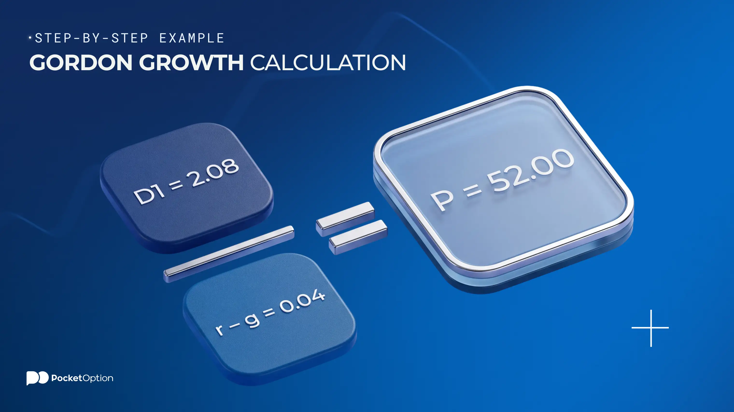
Assume a utility paid 2.00 per share this year. Dividend growth is expected to be 4% from here on, and the required rate of return is 8%.

1. Calculate the current dividend. D0 = 2.00.

2. Calculate D1, the growth of dividend by one year. 2.00 multiplied by 1.04 = 2.08.

3. Calculate the spread between the rate of return and the growth. 8% minus 4% = 4%, or 0.04.

4. Do the division. 2.08 divided by 0.04 = 52.00.

The model gives the valuation of 52.00 to the shareholder who accepts the three assumptions. Investor with different assumptions will get another number and both are right in their calculations.

You should check the answer in reverse. Rearranging the formula you get that the return is the sum of dividend yield and the growth rate: 2.08 divided by 52.00 is 4%, adding the 4% growth you get the 8% rate you began with. If that check fails, there is a miscalculation somewhere in the four steps.

How Changing r Affects the Result

Keep D1 = 2.08 and g = 4%, and change the required rate of return one percentage point at a time.

Single percentage point above or below the baseline shifts the valuation by twenty to thirty percent. Nothing has changed in the company in the table above. All that changed was your opinion of the return you should get from ownership of that share.

The reason is in r being present in the denominator only, and denominator is small. 4% spread means that you divide by 0.04, so the change of 0.01 is quarter of the whole divisor. The narrower the spread, the more violent the effect, so this model is the least reliable exactly where growth sits closest to the required return.

How Changing g Affects the Result

Now keep r at 8% and change the growth assumption instead. Notice that change in g implies change in D1 since the next dividend is increased by the same growth rate.

Two points of additional optimism double the valuation. It is even larger change than we got from the change in r because g affects both parts of the fraction: it increases the numerator slightly and decreases the denominator considerably.

The same equation can be rearranged and solved for the growth. The gordon growth rate formula states that g = r minus the dividend yield. At 52.00 price, 4% dividend yield and 8% rate of return, market expects the 4% perpetual growth. Solving the formula in reverse is often much more useful than solving it forward because it transforms the quoted price into the testable assumption: you stop asking what is the value of the share and ask whether 4% perpetual growth seems plausible to you.

What the Result Means: Overvalued vs Undervalued

Let's assume the calculation yielded 52.00 and the price is 44.00. The natural interpretation is that the market underpriced the share by eight dollars.

The disciplined interpretation is different. The difference tells us that our assumptions and market's assumptions contradict each other, and does not tell us which is right. Going back from the 44.00 with the same 8% required return you get market expectation of about 3.3% growth, not 4%. So the entire difference consists of 0.7 percentage points in an unverifiable number.

Expressed in this way, the result is the question rather than the conclusion. Why do we expect a growth the market doesn't expect? If we have a reason, such as a contract, a tariff decision, or a capital program underestimated by the market, we have a case. Otherwise, if the only reason we have is the spreadsheet, we have rounding error wrapped in the conclusion. This is the discipline which separates the valuation case from superficial interpretation, and it applies to fundamental analysis of stocks in general, not just to dividend valuation.

There is also the issue of actual prices behavior in the short term. Intrinsic value formulas say nothing about the timing, and a share may trade below the estimate for years. If the mechanism of quote formation and order matching is unfamiliar to you, there is a plain description of how the stock market works you should read along with this article.

Limitations of the Gordon Growth Model

The limitations are specific and not general, and each of them tells where the model loses sense.

• Constant growth is a fiction. No dividend has grown at fixed rate forever. Companies reduce payouts in recession, keep them constant for years and increase them in steps. The model smooths all of them to a single number and then compounds it forever.

• Extreme sensitivity of inputs. Two tables above show the valuation shift of twenty to thirty percent with one percentage point of change in r, and double with two points of g. Precision of the output is no proof of precision of inputs.

• Doesn't work with non-dividend paying companies. A company without dividend stream has zero D1 and the model gives you zero as the result, which is not informative.

• Ignores buybacks. Company returning money through buybacks instead of dividends is always undervalued by this method, and buybacks constitute a considerable part of distributions in several countries now.

• Assumes the rate of return is constant. While the rate in practice varies with interest rates and current level of risk of the business.

• Cannot handle a growth phase. Anything growing faster than its required return needs multi-period model for valuation, which uses gordon growth formula only in the final phase.

The companies where this model is applicable are mature, regulated and predictable: utilities, consumer staples and REITs. REITs are a particularly good match for it as the US REIT has to distribute at least 90% of its taxable income to shareholders in order to maintain tax status. If you are not familiar with this structure, there is an introduction to REITs and trading related stocks that covers how they are set up.

None of this makes the model useless. It simply limits its applicability to a particular type of companies, and leaves it as a thinking tool elsewhere.

Conclusion

Run it backward before you run it forward.

Use the price, dividend and the required return you can justify to find the growth rate implied by that price. You get one number to discuss instead of three, and the number you can prove by checking the actual behavior of the company: its history of dividends and payouts, reinvestments, industry growth rate. Running it forward, the model provides the value which looks like an absolute and relies on the assumptions never questioned. Running it backward, it gives you the question which can be answered. Same formula, and a much better use of it.

Disclaimer: This article is provided for informational purposes only and does not constitute investment advice. Trading and investing involve significant risk of capital loss, and valuation models rely on assumptions that may not hold, so they cannot predict future prices or returns.