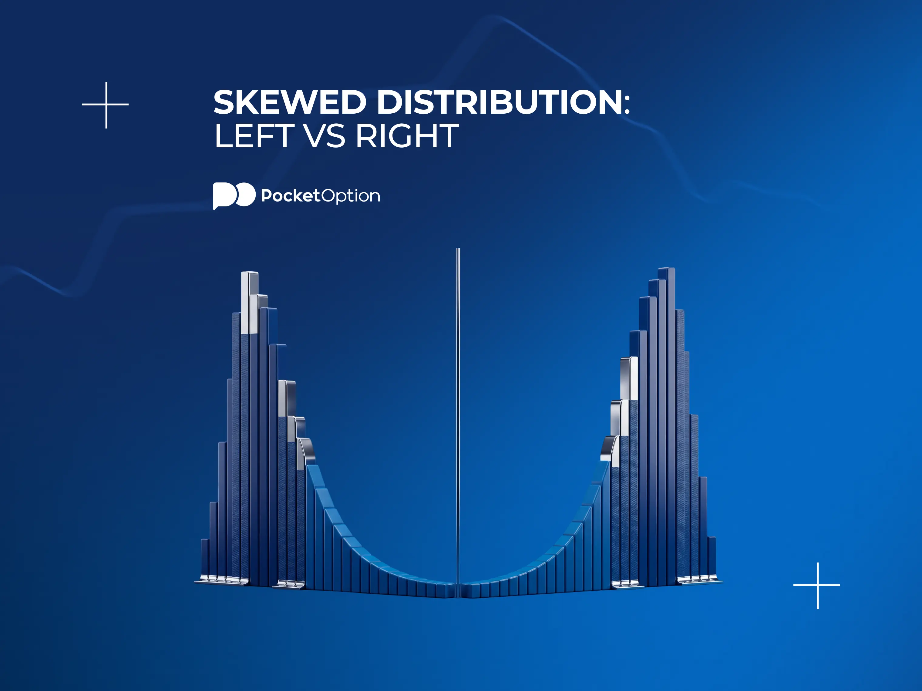
Skewed Distribution: Left-Skewed vs Right-Skewed Graphs

What Is a Skewed Distribution: Definition

A skewed distribution is not symmetric. If you fold it in half, the two halves won't coincide. One is extended into a tail, and the direction of that tail is what defines a distribution.

So the skew left vs right question is relatively easy to resolve, although many people tend to mix these two terms up in the process. Skewness is a measure of the asymmetry of the distribution, and it is named after the long tail, not after where the bulk of the probability lies.

So for instance a right skewed distribution, even though most observations are gathered on the left, is a distribution whose tail stretches to the right, and the name stems from this feature.

For the trader this means the following: skewness shows whether the extreme outcomes are going to be losses or gains. Two strategies can have the exact same average return, the exact same level of volatility, but completely opposite skewness, and this only manifests itself once something unusual occurs.

Right-Skewed (Positively Skewed) Distribution

As we've just learned, a right skewed distribution is a distribution whose tail points to the right. Most values are on the left, and some very large values create the tail and make the distribution extend in this direction.

Household income is probably the classic example. Almost everyone earns within a narrow interval, but a relatively small number of people earn an extraordinary lot, and that group pulls the average well above what the majority of people earn. Plotted as a skewed right histogram it will thus look like a tall bar on the left with a thin trail extending to the right.

In other words, the skewed right meaning is that the typical outcome is modest, and the exceptional one is exceptional precisely because of its magnitude. The losses are either rare or modest, but the gains are not capped in the same way and are occasionally very large.

In addition to the tail direction, there is another criterion for determining which skewness is present, and in a right vs left skewed comparison it is the peak position. For a skewed right graph, the peak is located on the left of the midpoint. The bulk of the probability lies below the average, and this might seem to be a disadvantage, but considering the reasons for the distribution taking such form, it's far from being so.

Left-Skewed (Negatively Skewed) Distribution

A left skewed distribution is the reverse. The tail points to the left, most values lie to the right, and some extremely poor outcomes pull the distribution left.

The age at death in a developed country is a good example. People tend to die in old age in a relatively narrow age bracket, but a minority dies considerably earlier. This makes the distribution left skewed, and a skewed left histogram looks like a thick bar on the right, with a long thin tail stretching toward zero.

This is a very dangerous form of skewness for a position holder. The skewed left meaning in practice is that things will generally work alright, and perhaps slightly better than average, but from time to time something goes horribly wrong, making the loss vastly disproportionate to the gains that preceded it.

It is a common distribution type in financial markets, and therefore the one to look out for, because the strategy that generates such a distribution might appear to perform superbly until the tail materializes.

Mean vs Median: The Key Giveaway

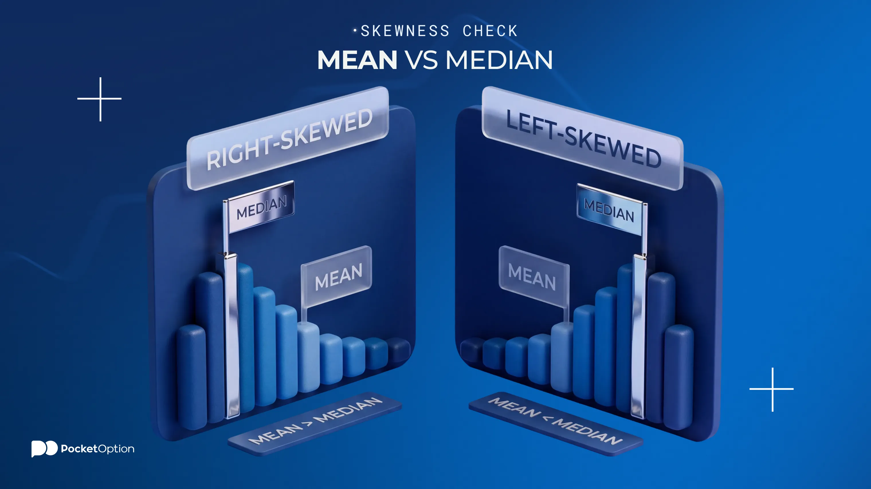
You often do not need a chart to get a sense of which way a dataset skews. Comparing the mean with the median gives you a quick indication, and it is a useful first look rather than a definitive test.

The reason is that the mean is affected by outliers, whereas the median is not. The median is the middle value after sorting, so a single extremely large outlier moves it one position, while the same outlier could move the mean quite a bit.

Thus, when the mean return of a dataset sits noticeably above the typical return, that usually points toward a right skewed distribution. When it sits below, that usually points toward a left skewed one. Treat these as indications rather than proof. The relationship holds for most ordinary unimodal data and there are known exceptions, particularly with discrete or multimodal distributions, where the comparison points the wrong way. If the answer matters, calculate the skewness statistic itself and look at the shape rather than relying on two summary figures.

This is worth applying to the records of your own trading. Find the mean and the median return per trade. If the mean sits well below the median, that is a signal worth investigating, and a small number of outsized losses is one common explanation among several. Check the actual distribution of your results before concluding which one applies to you.

Zero Skewness: The Symmetrical Case

A skewness reading of zero means the measure of asymmetry has cancelled out. In the common case that corresponds to a symmetric distribution, and the normal distribution is the classical example, with mean, median and mode all at the midpoint. It is worth knowing that zero skewness does not strictly guarantee symmetry. A distribution can produce a skewness of zero while still being asymmetric, if the deviations on each side offset one another in the calculation.

In actual samples you will rarely see exactly zero anyway, since random factors create tiny non-zero readings even in data drawn from a symmetric distribution. A value close to zero is interpreted as approximately symmetric, not as a mathematical guarantee.

The advantage of symmetric distribution is the intuitive nature of its standard deviation. Both losses and gains are of equal likelihood and equal in magnitude, so a single spread figure shows everything you need. Once skewness is involved, however, this convenience is lost.

Real Examples in Investment Returns

Both forms of skewness are observed in financial markets, and it is crucial to distinguish which one your strategy generates.

Positive skew: venture capital, buying options

Venture capital is the best known case. The majority of investments in a portfolio give a negligible return, some give a moderate return multiple of the investment, and one or two deliver a very large profit sufficient to carry the whole portfolio. The mean outcome is much better than the typical one, and that's how a positively skewed return series looks.

• Similarly shaped are the returns when buying options. The maximum loss here is the option premium paid, but the gains, if the price move went your way, are not capped in the same manner.

• Similar is the behaviour of trend-following strategies. Many small losses while the market trends sideways, then occasionally a large gain from the establishment of a trend.

• Lottery-like positions on small cap stocks are positively skewed as well, but there's a separate question of the expected value.

The problem with positive skewness is psychological. You spend most of your time in the small loss territory, while the profit that justifies the strategy still hasn't arrived, and many people quit just before the profit.

Negative skew: selling options, equity market crashes

Selling options reverses this structure. Here the premium is collected regularly, the position expires worthless the majority of times, and the income accumulates. Then the move occurs which is too large to be compensated by the premium collected so far, and one single event destroys a string of small profits.

• Equity market returns are negatively skewed. Declines are faster and larger than advances, and that's why on the chart of daily returns the left tail is longer than the right.

• Carry trade in currencies demonstrates the same feature. Interest differentials are steadily accumulated, then suddenly reversed with a violent move of the exchange rate.

• By design credit strategies show skewness in the same way. You earn the spread until the debt is defaulted, and then the loss overwhelms the profit collected up to now.

The measurement problem with negatively skewed returns is that all the usual measures of performance flatter them. Smooth returns, low volatility and excellent risk statistics are presented, because the event that defines the whole strategy hasn't occurred in the sampling period yet. Conventional risk statistics share this flaw, and this problem is discussed in this piece on how traders estimate potential portfolio loss with VaR.

What Causes Skewness in Returns

There are four mechanisms producing skewness in returns, and they usually act together rather than individually.

The first one is the payoff structure. Any financial instrument with asymmetric payoff structure produces asymmetric returns right away. Buying an option makes the downside limited while the upside is not capped in the same way, so the return series inherits this structure. Selling the option produces the opposite.

Leverage is the second mechanism. Positions are closed due to price movement rather than any decision to close them, and forced selling accelerates price declines in a way no forced buying could accelerate advances. One of the reasons of rapid declines and slow rises on equity market is precisely this mechanical effect.

Behavioral effect makes the third mechanism. Fear is faster than greed. Participants exit the positions simultaneously during stress and join the positions slowly during calm, so the result is rapid declines and gradual rises, and thus negative skewness in equity markets is an inherent characteristic rather than an occasional one.

The fourth mechanism is liquidity. In stressful times buyers stop coming in when their participation is most needed, so the same selling volume moves the price farther than on regular days.

Skewness vs Kurtosis

Kurtosis is often confused with skewness, but they are quite different measures of a distribution. Skewness describes which side the long tail sits on. Kurtosis describes how much weight sits in both tails combined, regardless of direction.

 Both measures are needed for full description of the return series. Typically the returns of an equity market index are negatively skewed and have high kurtosis, meaning that the extreme events are more frequent than a normal distribution allows and are concentrated on the negative side. Such a combination is far worse than any of the properties individually.

Why This Matters Beyond Standard Deviation

Standard deviation treats a gain and a loss of equal size equally. For someone who holds a position, they are quite different.

This creates a peculiar blind spot of standard deviation. Two strategies can have equal average returns and equal volatility, while being opposites in all other respects:

• The positively skewed strategy makes small losses frequently and gains very large amounts rarely. The worst realistic outcome of it is a long stretch of moderate underperformance.

• The negatively skewed strategy makes small gains frequently and loses large amounts rarely. The worst realistic outcome is losing a considerable share of your funds quickly.

• Both produce the same standard deviation. Only one of them can end the life of your strategy on the market.

Measures of risk-adjusted returns based on standard deviation have the same drawback. A negatively skewed strategy will show an excellent ratio for most of the period before the tail occurs, because there is no way of showing a loss which has not yet happened. It is not the fault of mathematics, it's the consequence of making the assumption of symmetry, explained in the guide to reading the bell curve and standard deviation.

The practical solution is to consider the skewness alongside volatility rather than instead of it, and to treat the smooth equity curve of a negatively skewed strategy as a red flag, not a green light.

Conclusion

Compare the mean return with the median return of your trading results before you look at anything else.

That single comparison gives you a first read on the shape of what you are doing, and the shape determines what a bad month can cost you. A mean sitting well below the median is a signal to look closer at your distribution of results, since a handful of outsized losses is one explanation and not the only one. If the mean sits above, you are likely running something positively skewed, and the danger is quitting during the long stretch before the payoff arrives. Volatility shows how much the returns move, but skewness shows from which side you can expect surprises, and that is the measure that decides whether you are still trading afterwards..

Disclaimer: Trading involves significant risk of capital loss and may not be suitable for all investors. Statistical measures reflect past data and do not predict future price behavior, and no risk framework excludes the possibility of loss.