Coefficient of Variation: Comparing Risk Across Assets of Different Scale

What Is the Coefficient of Variation: Definition

So what is the coefficient of variation? It’s the spread of a set of numbers, held up to the average of that same set. It’s written out as one ratio, and used by statisticians, investors and traders (although the first ones often call it ‘relative dispersion’). Traders say it is the ‘risk per unit of return’. Where lower is generally better.

The coefficient of variation definition is that it’s standard deviation, split by the mean. What makes it useful is that the units cancel. Dollars over dollars leaves a bare number. Percentage over percentage, same. That bare number is apt to sit next to any other bare number, 1 to 1, without an argument about scale or other metrics. You can compare apples to oranges, directly, just this once! And say which ones are probably more risky to invest in.

Once you’re actually holding and comparing two assets in front of you, what does coefficient of variation mean? It means you’ve stopped asking how much a thing moves. You’re now instead asking how much it moves per unit of return you can get out of it. CV of 0.5 says the average swing is half the size of the average outcome. It’s suitable for long-term investing. Compare it to the asset with a CV of 2, where the swing is twice that size, which is a different animal entirely, a much riskier one. This is a high-risk speculation, or is suitable for a daytrader looking for massive swings.

Coefficient of variation meaning does not shift about when you carry it between fields. Biologists put it on cell counts, engineers on tolerances, and CV statistics turn up no end of times in quality control work. Finance merely borrowed the thing. So what is a coefficient of variation good for? Setting two unlike things side by side, and not letting anything extra get in the way!

Why Standard Deviation Alone Isn't Enough to Compare Assets

Put two shares next to each other. First one trades around 800 a unit and its price wanders with a standard deviation of 40. Second one sits at 20 and wanders by 2. Raw figures say the first is twenty times the handful, but that reading is wrong (or, rather, wrong enough to cost you real money).

Split each by its own average and the picture flips over. 40 over 800 comes to 0.05. 2 over 20 comes to 0.10. Per unit of price, the cheap share now is doing twice the moving, and nothing in the standard deviation column was ever going to say so. This is why coefficient is important, and useful.

Same trap shows up with currencies, and in a lot of other places in finance. A fund reported in yen carries a standard deviation with a great many more digits in it than the same fund reported in euros, but those extra digits tell investor/trader nothing about risk.

Standard deviation, of course, is still worth having, and you can read this walkthrough of deviation trading and market analysis to see why. But problem starts the moment the two things being measured sit on different scales to begin with.

The Coefficient of Variation Formula

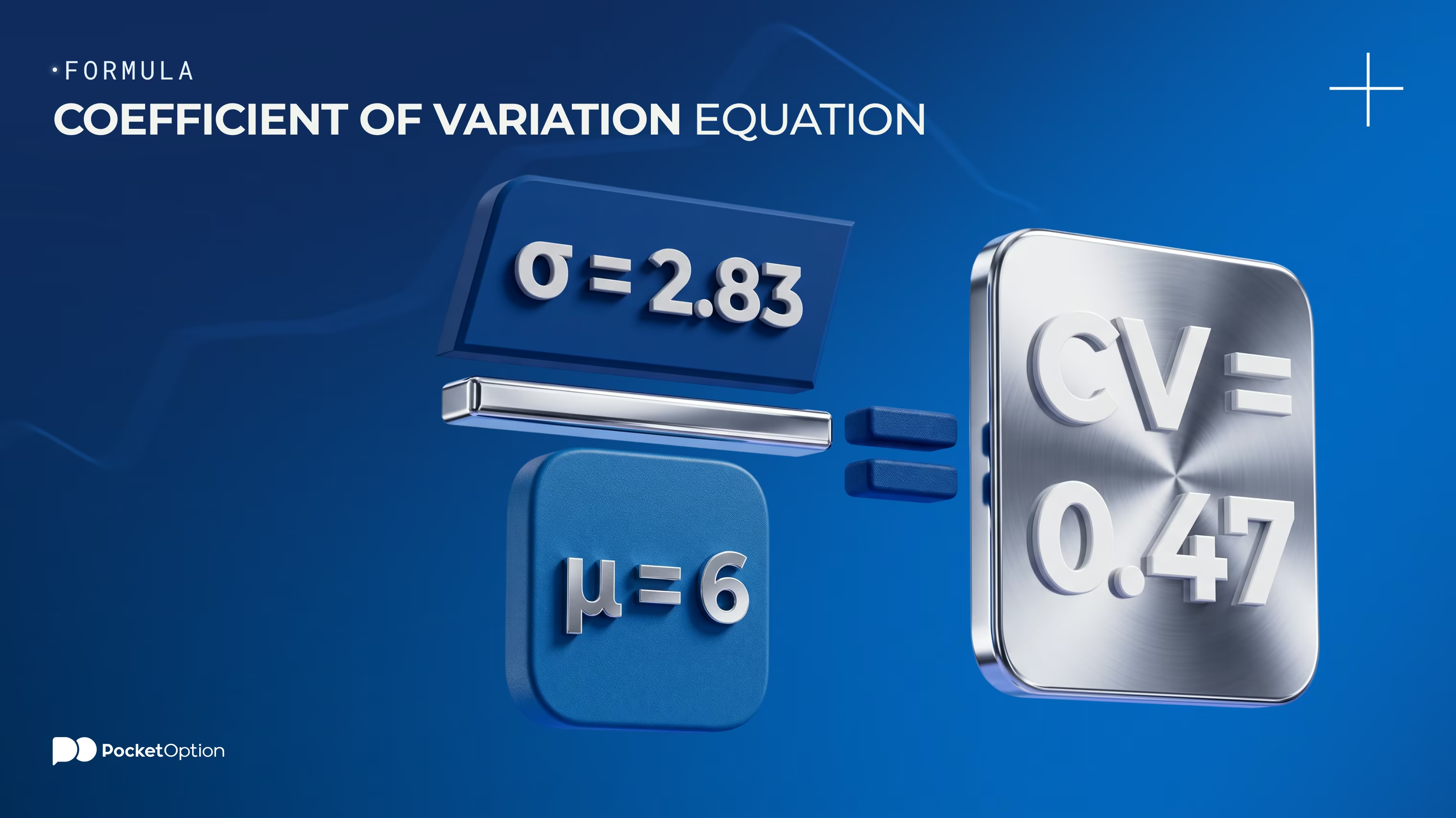
First question is what is coefficient of variation, and second one is how to work it out. In actuality, the coefficient of variation formula is short in pretty:

CV = σ / μ

σ here is the standard deviation, and μ is the mean. That is the whole story.

Written in plain english, the formula for coefficient of variation reads: standard deviation split by the mean. You can also multiply what comes out by 100, of course, if you want it as a percentage. Some textbooks also write the coefficient variation formula with the percent already baked in, so CV = (σ / μ) x 100, and both versions are the same sum. The short CV formula and the percentage one don’t disagree, one is merely scaled up a hundredfold, for ease of reading.

Two cautions attach to the coefficient of variation equation before any numbers go into it. Mean and standard deviation have to come off the same data, over the same window, in the same units. And the mean wants to be positive and not sat too close to zero, for reasons the caveat section further down gets into.

From Variance to Standard Deviation to CV: Step by Step

Variance, standard deviation, CV, they all come out of the same handful of numbers. As an example, let’s take five annual returns: 4%, 8%, 2%, 10% and 6%.

1. Work out the mean. Here, 4 + 8 + 2 + 10 + 6 = 30, split by 5 (total amount of years),  the mean ends up being 6%.

2. Take each return away from the mean. You come by -2, +2, -4, +4 and 0.

3. Square each of those and add them up. 4 + 4 + 16 + 16 + 0 = 40.

4. Divide by 5 for the variance of the whole set, which gives 8. Units here are percent squared, a quantity nobody has ever had an intuition about.

5. Square root of 8 is roughly 2.83, and that is the standard deviation. Split it by the mean of 6 and the CV lands at 0.47, or 47%.

Worked Example: Comparing Two Market Indices

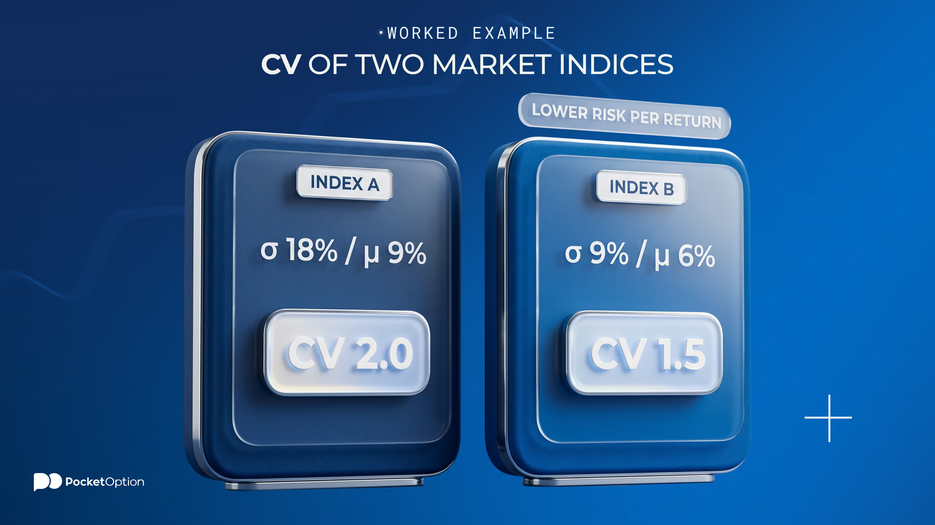
Let’s take two indices: index A has averaged 9% a year with a standard deviation of 18%. While index B has averaged 6% with a standard deviation of 9%. Which is better to invest in? Many investors would say A, as the return seems higher, and they wouldn’t think much more about it.

But let’s run the math. On standard deviation alone, A is the rougher ride, twice as rough. On return alone, A is the better payer, half again as good. Neither column settles anything, they merely argue with each other.

Run the CV and the argument stops. A gives 18 / 9 = 2.0. B gives 9 / 6 = 1.5. Remember, lower is better. So B is carrying less turbulence for every point of return it spits out. If you want less risk associated with holding, it might be a better choice of the two.

This doesn’t make A the wrong holding, it’s just different. An investor who can sit through wider swings and wants the higher average may well take A on purpose, losses and all. What the CV does is stop anyone pretending the extra 3 points of return came free.

Worked Example: Comparing Two Hypothetical Investments

Second case, and here the returns match exactly. Investment X has averaged 2% a month with a standard deviation of 3%. Investment Y has also averaged 2% a month, standard deviation 1.6%.

Same return. Not the same investment. X works out at 3 / 2 = 1.5. Y works out at 1.6 / 2 = 0.8, a shade over half of X. Whoever held Y got to the same place with a good deal less lurching on the way there, and the lurching is the part that empties accounts early, since a drawdown deep enough forces the sale before the average ever arrives.

CV will not tell you how deep that drawdown might run. For the depth question there is a separate tool, and this explainer on value at risk and potential portfolio loss handles it properly. Read the two together and you come away holding both the shape and the worst case.

Coefficient of Variation vs Variance

Variance is the first step of the sum, not a rival to the last one. It is the average of the squared deviations, and because the squaring happened it is sat in units nobody can picture. Percent squared. Dollars squared. Try explaining a dollar squared to a client.

Coefficient of variation is the far end of the same chain, after the square root has undone the squaring and after the division has knocked the units out altogether. Variance is good for the maths that comes after it, portfolio work expressly, where the variances of combined holdings behave better than standard deviations do. CV is good for comparisons. Different jobs, same family.

Coefficient of Variation vs Standard Deviation

These two get muddled oftener than the rest, which is fair, seeing as one is built straight out of the other. Difference is what sits underneath each.

• Standard deviation answers how far from the average this thing usually strays, in the units you started with.

• CV answers how far it strays relative to the average itself. No units left.

• Standard deviation is absolute risk. Handy when the two things being weighed already sit on the same scale, same currency, roughly the same price.

• CV is relative risk. Or risk per unit of reward, if you would rather put it that way.

• Where the means are near enough identical, both measures rank assets the same way and either will do. Where the means diverge, only one of them is still telling you the truth.

Neither one is a forecast. Both are built out of what already happened, and a quiet asset is under no obligation to stay quiet.

What a Lower or Higher CV Tells You

Lower CV means less dispersion for each unit of average return. Higher CV means more of it.

What it does not mean is that low is good and high is bad, full stop. A CV of 0.4 on an asset averaging 1% a year is a very steady way of going almost nowhere. A CV of 2.5 on something averaging 30% might suit a small slice of a portfolio that can afford to be wrong, and the losses in that slice can run to the whole of it. CV ranks the trade-off. Choosing where on that trade-off you want to sit is a separate decision and it belongs to you, not to the ratio.

Rough handling rule: compare CVs only amongst assets you would genuinely hold for the same purpose, over the same window, measured the same way. Cross-window comparisons are where the number turns into decoration. Monthly figures set against annual figures will mislead every time, because the mean scales with time in one manner and the standard deviation in another.

Caveat: When CV Becomes Misleading

Denominator is where the whole thing breaks. Push the mean toward zero and the ratio runs off toward infinity, so an asset averaging 0.1% with a standard deviation of 5% shows a CV of 50, which reads like catastrophe and is really just a very small number sat underneath a fairly normal one.

Negative means are worse again. A loss-making average spits out a negative CV, and negative CVs cannot be ranked against one another in any way that means anything at all. Most practitioners simply refuse to report one. Sensible.

There is a scale condition too, and it gets almost no airtime. CV wants a ratio scale, meaning a variable with a true zero underneath it. Temperature in Celsius has no true zero, so the CV of a run of Celsius readings changes the moment you convert those same readings to Fahrenheit, which rather gives away that the statistic was never measuring anything real there. Returns and prices are fine on this count. Not everything is.

Last one, and it is the one that costs money. CV says nothing whatever about the shape of the distribution. Two assets can share a CV and carry wildly different tails, and it is the tail that does the damage. Working through how to read the bell-shaped curve and its standard deviation percentages fills that gap in, and it is worth doing before leaning on any single dispersion figure. Small samples deserve a mention as well. Twelve monthly returns will hand you a CV. They will not hand you a reliable one.

Conclusion

Use CV on assets you are weighing for the same job. Check that the mean is positive and not tiny, before trusting whatever comes out. And keep the standard deviation in view alongside all of it, because knowing an asset is twice as variable per unit of return still leaves you needing to know how much money that is in absolute terms, and money is what gets lost.

Disclaimer: Trading involves risks of capital loss and may not be suitable for all investors. Past performances do not guarantee future results.