Sharpe Ratio Explained
Two traders finish the year with 20% gains. Same number, very different stories. One built that return through dozens of small, consistent wins. The other survived three near-wipeouts to get there. Which account would you rather manage? The sharpe ratio is the metric that separates these two situations, putting return and volatility on the same scale so the comparison becomes honest. Most traders encounter this ratio at some point, nod along, then go back to looking at returns. That is a mistake. Once you actually understand what the number measures and where it breaks down, you start reading strategy results very differently.

What Is Sharpe Ratio?
Developed by economist William Sharpe in 1966, the ratio captures one thing: how much return a strategy generates for each unit of risk it takes on. Not gross return. Not percentage gain. Return per unit of volatility.
Want to test your strategy without risking real capital? Open a free demo account and track your results across 100+ assets
Open Demo AccountHere is the key distinction. A strategy that earns 15% with very stable monthly results scores far higher than one earning 15% through violent swings. Both hit the same annual number. Only one of them required the trader to sit through frightening drawdowns to get there. The ratio makes that difference visible in a single figure.
Traders and portfolio managers use it constantly, in fund reporting, backtesting, strategy comparison, and selecting which signals to follow. The number does not tell you whether an absolute return is impressive. It tells you whether the journey to that return was worth the turbulence involved. That is a completely different question, and arguably the more useful one for day-to-day decision-making about how to allocate capital.
Running a strategy through a pocket option demo account before committing real funds gives you the performance data needed to calculate meaningful ratios, real fills, real spreads, without capital at risk.
Why Traders Use Sharpe Ratio
The practical case for the sharpe ratio formula comes down to one recurring problem: raw return comparisons are misleading. If someone tells you their system made 30% last year, the only sensible response is to ask how volatile it was. A 30% gain built through smooth, consistent performance is completely different from 30% that required surviving a 45% intra-year drawdown. The ratio converts both into a single comparable number.
Traders use it in several specific ways:
Comparing strategies: Two approaches with similar returns often look very different once volatility enters the picture. The ratio forces that comparison to happen fairly.
Evaluating signal providers: A provider showing strong returns over 6 months tells you almost nothing. The same return over 3 years with a decent ratio is a genuinely useful data point.
Auditing backtests: Curve-fitted strategies tend to produce unusually high ratios over historical data that collapse in live trading. A suspiciously high number in a backtest is a red flag worth investigating.
Portfolio construction: Combining two assets with acceptable individual ratios and low correlation between them often produces a portfolio ratio higher than either asset alone. This is one of the core mechanics behind diversification.
Trading involves significant risk of capital loss. This article is for educational purposes only and does not constitute financial advice. Always conduct independent research and consider your risk tolerance before making any trading decisions.
Sharpe Ratio Formula
The mechanics of what is sharpe ratio sit inside a simple three-part calculation:
Sharpe Ratio = (Rp - Rf) / Op
| Component | What It Means in Practice |
|---|---|
| Rp (Portfolio Return) | The annualized return of the strategy or portfolio being measured. This is the total gain over the period, expressed as an annual figure. |
| Rf (Risk-Free Rate) | The return available from a completely safe investment, typically short-term government bonds. It represents the baseline return requiring zero market risk. |
| Op (Standard Deviation) | The annualized standard deviation of excess returns. This measures how much monthly or weekly returns deviated from their average, capturing volatility. |
The numerator strips out the easy part of the return, the portion anyone could have earned by sitting in government bonds. What remains is the true value added by taking market risk. The denominator then adjusts that number for how bumpy the ride was. Divide one by the other and you get a clean measure of efficiency.
How to Calculate Sharpe Ratio?
The sharpe ratio meaning becomes concrete through a worked example. Here are two real-world-style strategies with different characteristics:
Strategy A: Conservative trend system
Annual return (Rp): 16%
Risk-free rate (Rf): 4%
Standard deviation (Op): 9%
Calculation steps:
Excess return: 16% - 4% = 12%
Divide by volatility: 12% / 9% = 1.33
Strategy A result: 1.33
Strategy B: Aggressive momentum system
Annual return (Rp): 28%
Risk-free rate (Rf): 4%
Standard deviation (Op): 26%
Calculation steps:
Excess return: 28% - 4% = 24%
Divide by volatility: 24% / 26% = 0.92
Strategy B result: 0.92
Strategy B printed nearly twice the raw return. On a risk-adjusted basis, it underperformed Strategy A by a meaningful margin. For a trader managing risk carefully, especially with real money and real emotional responses to drawdowns, Strategy A is the stronger choice even though the headline return looks inferior.
What Is a Good Sharpe Ratio?
Understanding what is a good sharpe ratio requires a reference framework. These ranges are widely used, though context always matters:
| Ratio Value | What It Typically Signals |
|---|---|
| Below 0 | Negative risk-adjusted return. The strategy lost relative to the risk-free rate after accounting for volatility. |
| 0.0 to 0.5 | Poor. Returns do not adequately compensate for the risk involved. |
| 0.5 to 1.0 | Acceptable. Not outstanding, but reasonable for many active strategies. |
| 1.0 to 2.0 | Good. Solid efficiency, relatively difficult to sustain over multiple years. |
| 2.0 to 3.0 | Very strong. Rare in live trading; more common in backtests, which should prompt scrutiny. |
| Above 3.0 | Exceptional or overfitted. Almost always requires explanation in a live context. |
Professional fund managers typically land between 0.5 and 1.5 over multi-year horizons. Retail strategies consistently above 1.0 are performing well relative to their volatility. Numbers above 2.0 in a backtest are worth questioning closely, as overfitting to historical data is the most common cause.
Sharpe Ratio vs Other Risk Metrics
The sharpe ratio definition formula is not the only way to look at risk-adjusted performance, and it is not always the best choice. Two alternatives address specific problems with the standard calculation:
| Metric | Risk Denominator | Main Use Case | Key Advantage Over Sharpe |
|---|---|---|---|
| Sharpe Ratio | Total volatility (upside and downside) | General strategy comparison | Widely understood, easy to calculate and compare |
| Sortino Ratio | Downside volatility only | Strategies with large positive outliers | Does not penalize winning months that inflate standard deviation |
| Treynor Ratio | Beta vs market benchmark | Portfolio performance vs index | Better suited for portfolios measured against a benchmark |
The Sortino ratio solves a real problem. When a strategy occasionally produces very large winning months, those gains push up standard deviation and artificially lower the Sharpe ratio. Sortino only counts the months where returns fall below a minimum threshold. For trend-following strategies with positively skewed return distributions, Sortino is often the fairer measure.
Treynor is less relevant for pure trading strategies and more useful for evaluating traditional portfolios. It replaces standard deviation with beta, so it only captures systematic risk rather than total volatility. Most retail traders are better served by sticking with Sharpe and Sortino as their primary tools.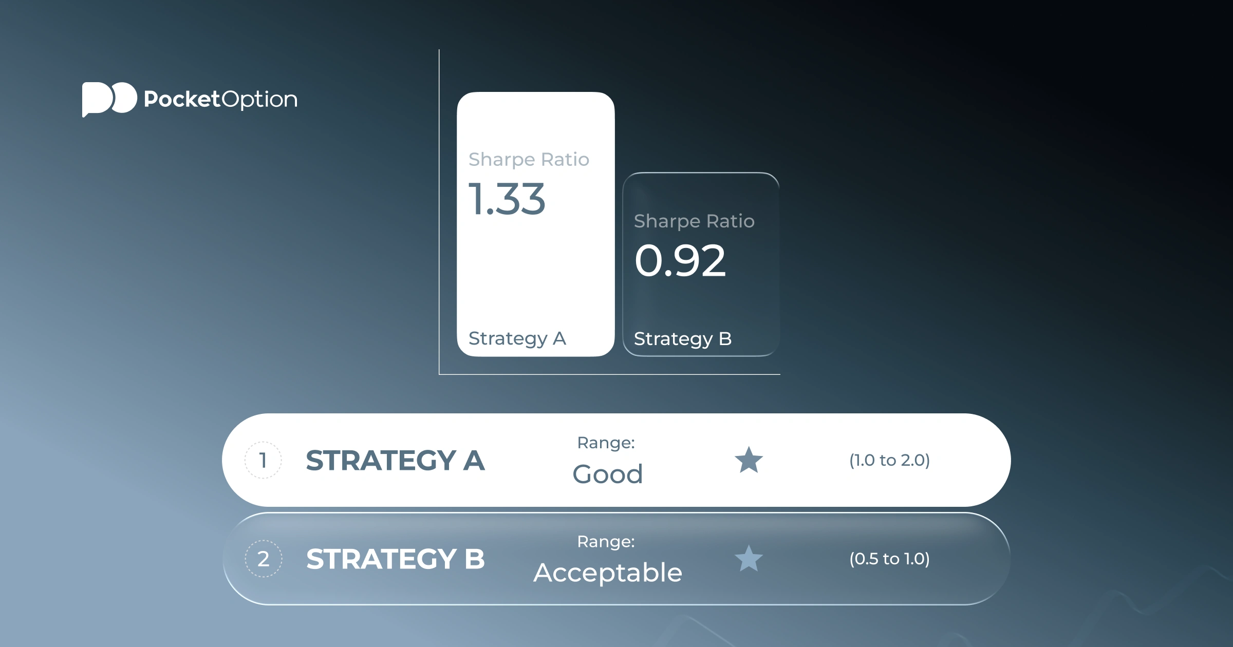
Limitations and Disadvantages
No single number captures everything. Anyone relying on the ratio without understanding its blind spots will eventually be surprised.
Returns are not normally distributed in real markets. The formula assumes that monthly gains and losses follow a bell curve. They do not. Crashes happen more often than the math predicts. A strategy can show a perfectly acceptable ratio right up until a tail event wipes out months of gains.
Good volatility and bad volatility are treated the same. A month where the strategy gains 25% raises standard deviation just as much as a month where it loses 25%. Strategies that win big in occasional months but lose small the rest of the time look riskier than they actually are in practice.
Short time periods are almost meaningless. A ratio calculated over 12 months can be driven almost entirely by a single favorable market regime. Three or more years of data is the minimum for anything resembling reliability.
Drawdown patterns are invisible. Two strategies with the same annual return and the same standard deviation can have completely different drawdown sequences. One might recover from losses in days. The other might spend six months underwater before recovering. The ratio cannot distinguish between them.
The risk-free rate shifts the output. In a high-rate environment, the same strategy generates a lower ratio than it would in a near-zero-rate environment, even if nothing about the strategy changed. Ratios calculated in different rate regimes are not directly comparable without adjustment.
The practical implication: use results from applying how to calculate sharpe ratio methodology as a starting point, not a conclusion. A strong ratio is encouraging. It does not replace checking maximum drawdown, recovery time, live versus backtest consistency, and the broader market conditions under which the performance was achieved.
Xem thêm:Glossary